The projects I enjoy most all involve visuals that anyone can easily understand from a high level viewpoint. An example is this maze project, which I worked with a team of two others to create in my AI class. This project involved working with mazes and using different types of search algorithms to solve them. My team showed how different algorithms found different paths through randomly generated mazes. The project also dealt with making mazes more difficult in an algorithmic way.
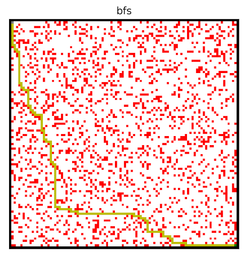
Breadth First Search
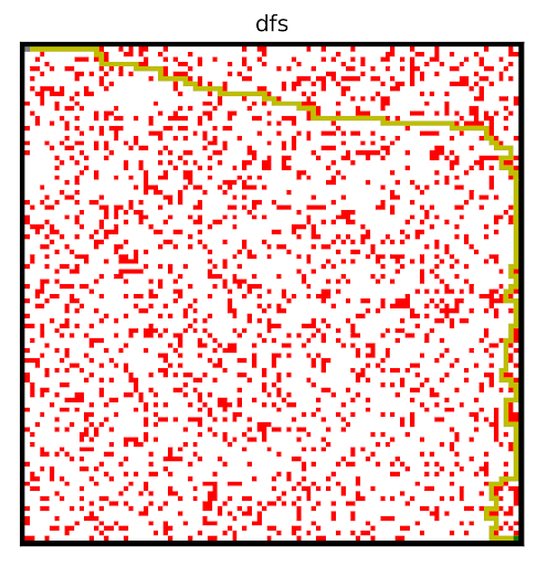
Depth First Search
Above, note the classic breadth first search and depth first search algorithms, ran on the same graph. Although not earth shattering, they are useful for comparison with other algorithms.
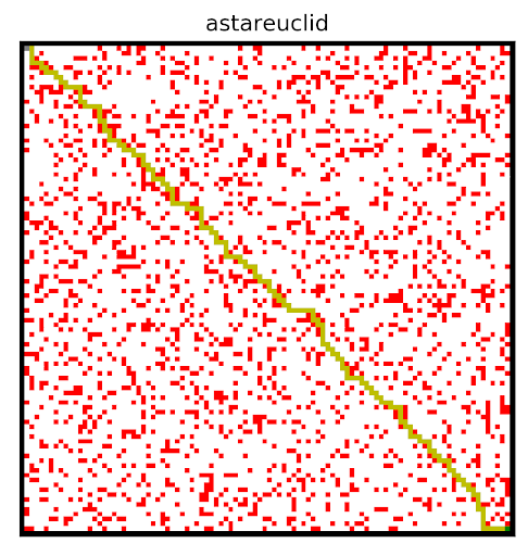
Informed Search using Euclidean distance
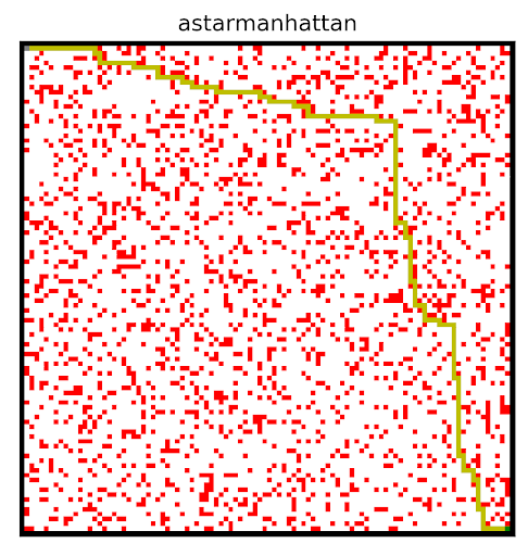
Informed Search using Manhattan distance
These results are prime examples of the usefulness of a good visualization. Both of the algorithms are informed searches, meaning that they pick their next move based off of the shortest distance. However they do so in alternate ways. Both of these algorithms calculate what the distance to the finish would be if they moved in any of the four possible directions. They then choose the direction with the lowest distance, and keeps track of its previous actions in case it gets stuck and needs to go back. Where they differ is in the method they use to calculate that distance.
Green- Euclidan distance
Red, Blue and Yellow- Manhattan distance
Image Source
The image above shows a few ways the agent could calculate distance. Something to note, that is hard to see,
is that all paths are the same length. But the reason why the agent discovered two equal but different paths can be learned
when we take a closer look at the method used to calculate the distances.
One method is to use a naive approach, and simply
measure the length of the direct path from a given square to the finish. This is shown by the green line,
and is known as Euclidean distance. However, this is not entirely accurate. The agent can only move up,
down, left and right and not in any angle it wanted. You can see the side effect of this in both the blue path in the example image
and when the agent used euclidean distance to solve the maze. The agent tried to stay as close to a diagonal path as it could.
Meanwhile, Manhattan distance assumes you can only move in the four cardinal directions and is a more accurate measure of
distance in this case. This caused the agent to follow a less direct path, something akin to the yellow line in the image above.
This path still requires the same amount of moves as the path discovered by the euclidean distance agent.
However, it highlights the difference between the two ways of measuring distance.
Another part of the project involved creating the hardest possible graph for a given search algorithm, by some measure of "difficulty". I used a search algorithm called beam search that experimented with inverting cells,
and incrementally made the graph harder and harder for a given search algorithm. In the two examples below, the algorithm searched for graphs that would be difficult for depth first search.
This resulted in interesting visuals, where the graph gets more and more complex over time.
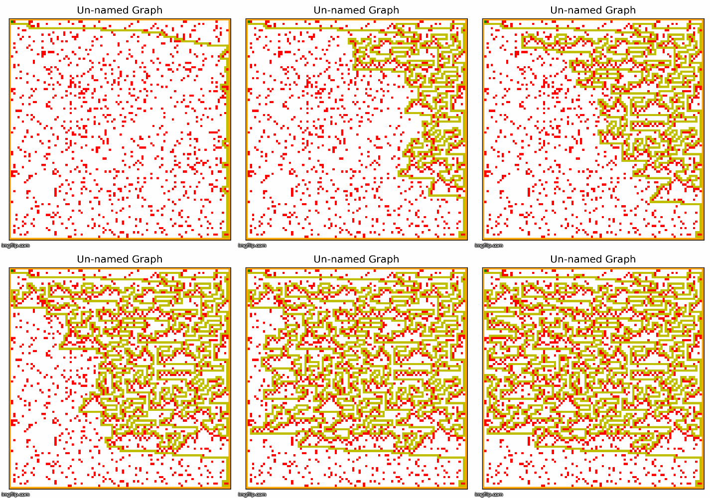
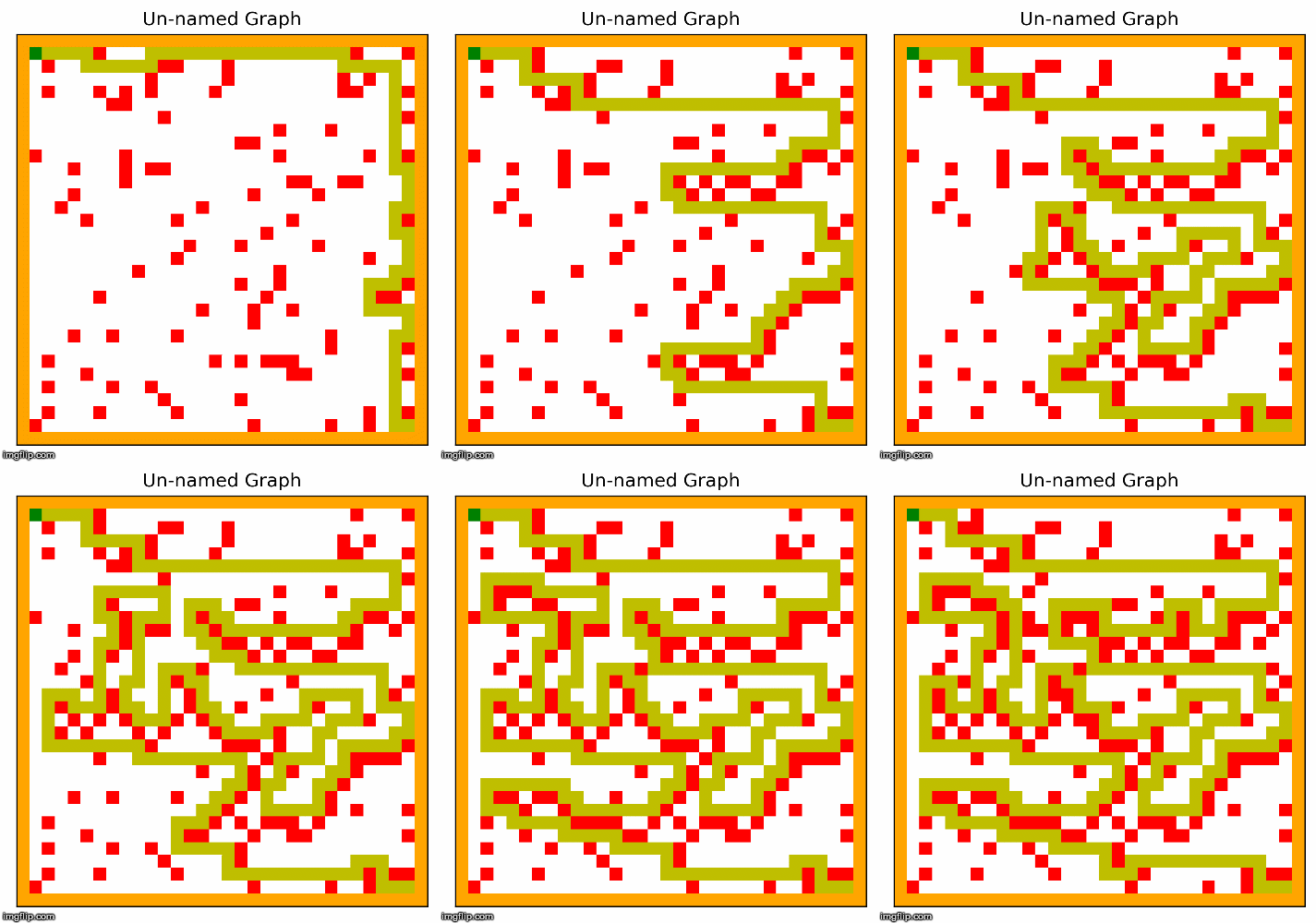
I particularly like these images! We can see the maze becoming more difficult to solve, as the computer places blocks to exploit the depth first search algorithm. Something to note about DFS is that it will go for as long as it can before backtracking and trying a different path, and if it finds the goal it will never backtrack. Our implementation of depth first search prioritizes going right, then down, then left, and lastly up. The reason why we settled on this heuristic was because most of the time, the goal would be down and to the right. So beam search exploits this by building mazes where going right most of the time is a bad strategy. I also think it is quite cool how beam search works with the original squares in the maze, connects them in to walls. The beam search algorithm figured all of this out by simply inverting random squares and seeing if that caused the path to become longer. It does not understand depth first search, or how our implementation prioritizes certain directions. Yet the end result looks as if it was produced by something that understands how DFS decides on the next move.